Spatial Autocorrelation
Spatial autocorrelation is a concept that refers to the degree to which the values of a variable are correlated in space. In other words, it examines whether nearby locations tend to have similar values for a particular variable. It is an essential concept in understanding spatial patterns and dependencies in data. Understanding spatial autocorrelation is crucial for making informed decisions in spatial analysis and modeling, as it provides insights into the underlying spatial structure of data and helps to identify spatial dependencies that may affect statistical inference and modeling assumptions.
For testing spatial autocorrelation, there are statistical methods used to assess whether spatial patterns in a dataset are significantly different from what would be expected. These tests help researchers determine whether there is evidence of spatial dependence or clustering in the data. One of these tests for spatial autocorrelation is Moran’s I.
Moran’s I test
Moran’s I is a global measure of spatial autocorrelation that quantifies the degree of similarity between neighboring observations in a dataset. There different types of this test, one of them is the Moran’s bivariate. This spatial test is an extension of Moran’s I that allows for the analysis of spatial relationships between two different variables simultaneously. It measures the degree of association between the values of two variables across spatial units, considering both the values of each variable and their spatial locations.
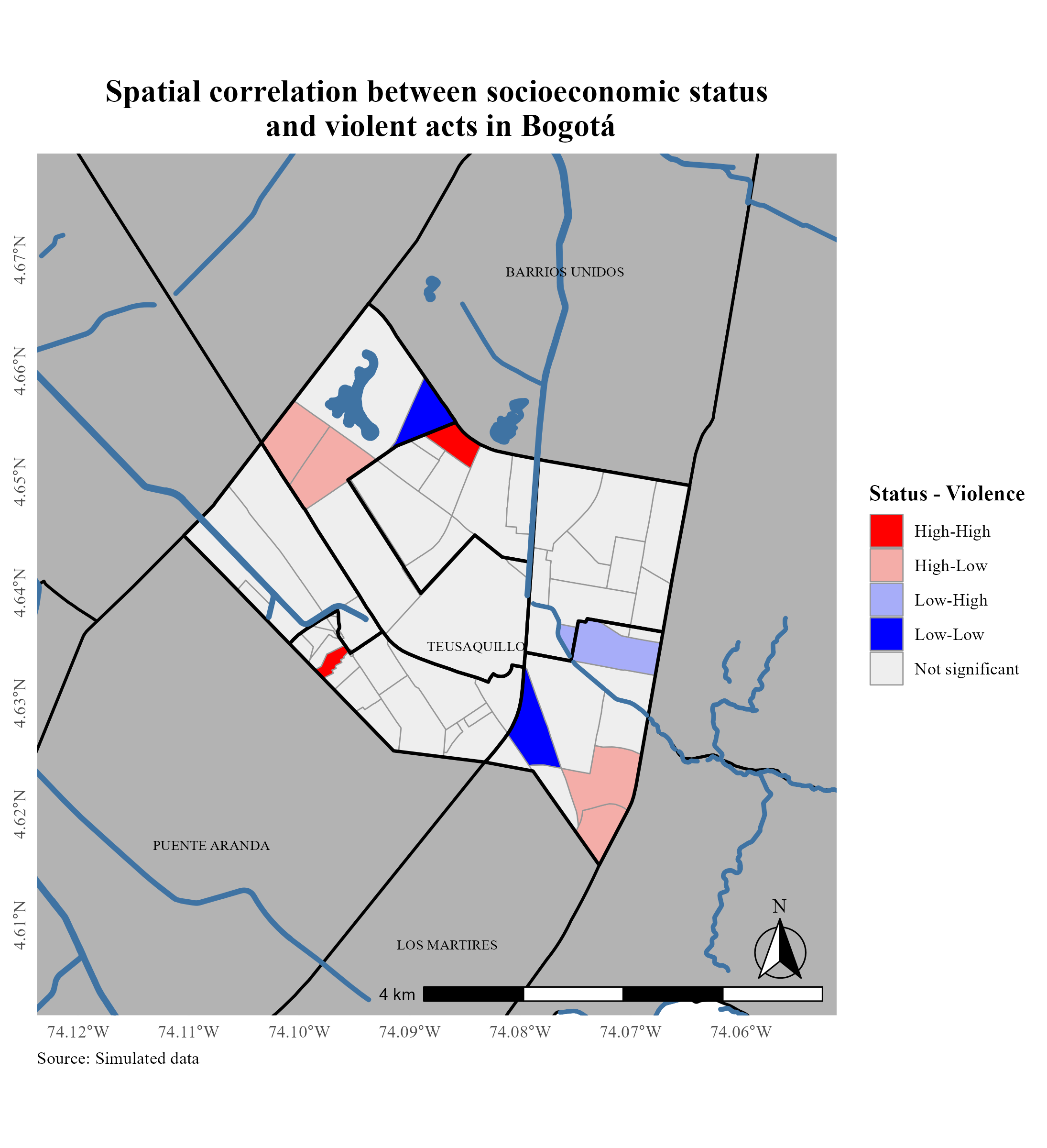
A study case in Bogotá
In order to make an example of this test, I simulated a database of socioeconomic status and violent acts in Bogotá focusing in Teusaquillo. The graph shows places with different socioeconomic levels in which acts of violence occur on different scales. For example, red areas have a high socioeconomic level but suffer from a high level of violence.
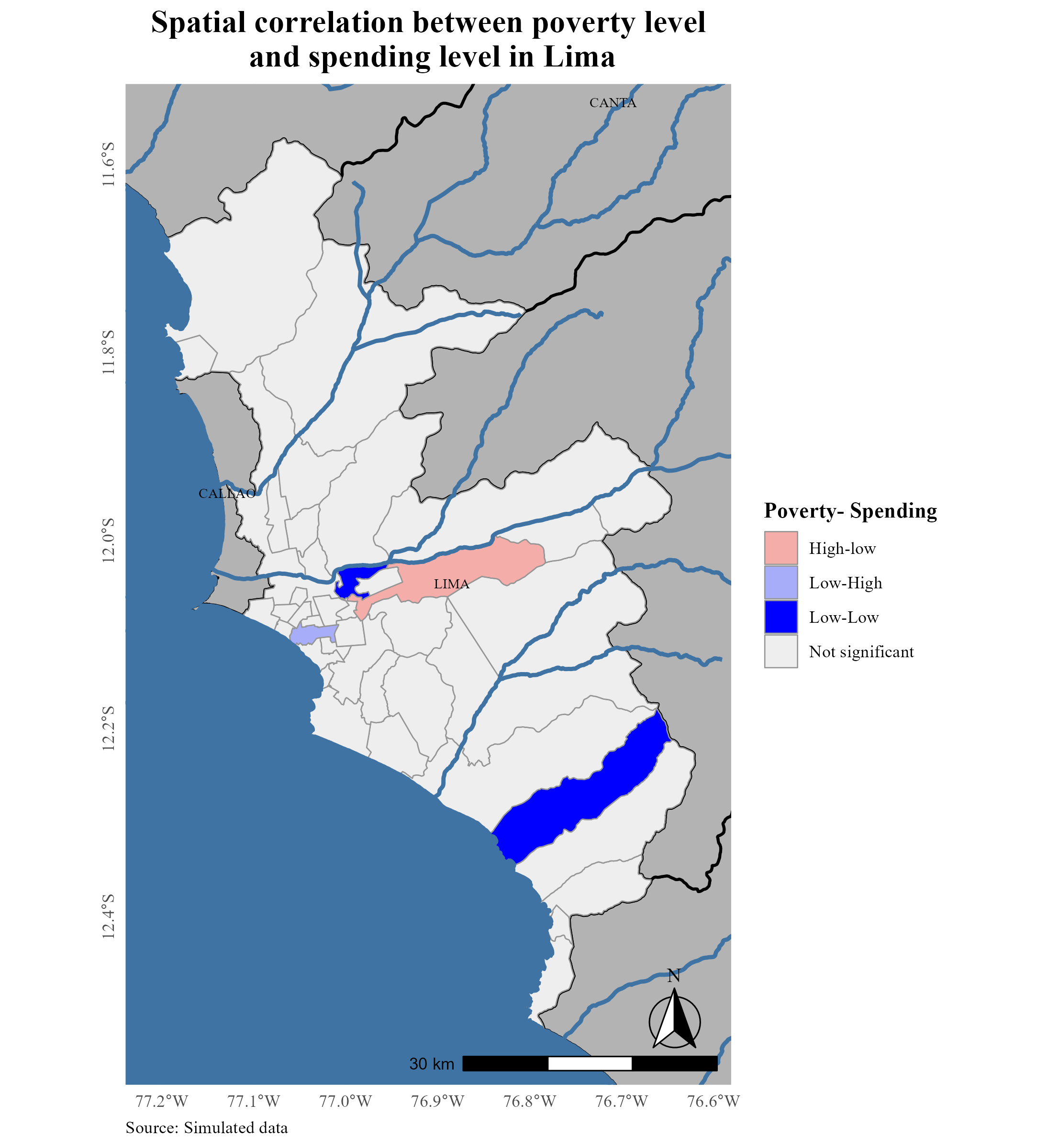
A study case in Lima
To continue with the examples, I simulated a databsae of poverty level and per capita household spending level for Lima. The administrative boundaries are in level 2. The way to understand the graph is the same than the last one. For more information regarding the commands used, please feel free to email me on p.valcarcel@uniandes.edu.co.